Example

In this example, we are going to solve the thermodynamically consistent electrolyte model for an incompressible, ternary electrolyte, as it is done in https://git.rwth-aachen.de/JanHab/fxdgm/-/blob/main/examples/ReproducableCode/TernaryElectrolyte.py?ref_type=heads.

Install the package and FEniCSx backend

pip install git+https://git.rwth-aachen.de/JanHab/fxdgm
conda install -c conda-forge fenics-dolfinx=0.8.0 mpich=4.2.1 pyvista=0.43.10 gcc=12.4.0 -y

Import the necessary libraries

# Import the fxdgm package
from fxdgm import solve_System_4eq

# Import the necessary libraries
import matplotlib.pyplot as plt
import numpy as np

Define parameters and boundary conditions

# Boundary conditions
phi_left = 8.0
phi_right = 0.0
p_right = 0.0
y_A_R = 1/3
y_C_R = 1/3

# Mixture properties
z_A = -1.0
z_C = 1.0
K = 'incompressible'
Lambda2 = 8.553e-6
a2 = 7.5412e-4

Define mesh and solver settings

number_cells = 1024
# Local mesh refinement towards the electrode
refinement_style = 'log'
# Relative tolerance for the newton solver
rtol = 1e-8

Solve the system

y_A, y_C, phi, p, x = solve_System_4eq(
    phi_left, phi_right,
    p_right,
    z_A, z_C,
    y_A_R, y_C_R,
    K, Lambda2, a2,
    number_cells, relax_param=0.05,
    x0=0, x1=1,
    refinement_style='hard_log', return_type='Vector',
    max_iter=1_000, rtol=rtol
)

Visualize the results

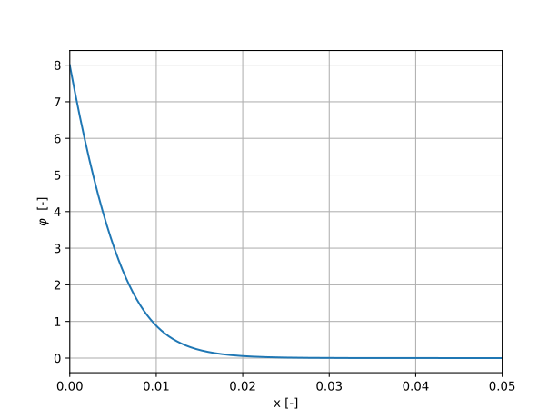
# Electric potential
plt.figure()
plt.plot(x, phi)
plt.xlabel('x [-]')
plt.ylabel('$\\varphi$  [-]')
plt.xlim(0,0.05)
plt.grid()
plt.show()

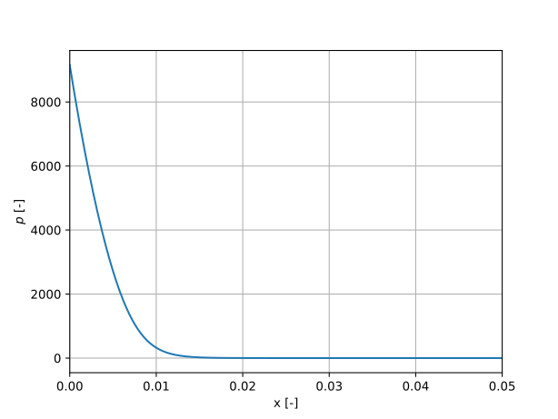
# Pressure
plt.figure()
plt.plot(x, p)
plt.xlabel('x [-]')
plt.ylabel('$p$ [-]')
plt.xlim(0,0.05)
plt.grid()
plt.show()

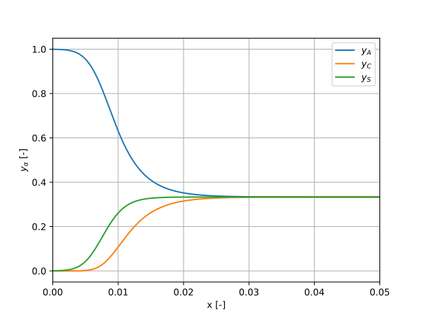
# Atomic fractions
plt.figure()
plt.plot(x, y_A, label='$y_A$')
plt.plot(x, y_C, label='$y_C$')
plt.plot(x, 1 - y_A - y_C, label='$y_S$')
plt.xlabel('x [-]')
plt.ylabel('$y_\\alpha$ [-]')
plt.xlim(0,0.05)
plt.grid()
plt.legend()
plt.show()

The electric potential

The pressure

The atomic fractions